Efficient Inverted Indexes for Approximate Retrieval over Learned Sparse Representations

Picture this. You have a rather large collection of (short) text documents. Passages from long legal or financial documents; snippets from novels; or articles from the web, are a few examples. Typically you are not just hoarding data for no reason. Instead, you have collected this data so that you can process it. One very routine example is to find information that is relevant to you, or can help you answer a very specific question.

Considering the sheer volume of massive collections, it would be nearly impossible to sift through all this data manually to find answers to your questions, right? That is why “search” has become such an indispensable tool that we rely on daily. We have a question (a “query”) and we wish to find, from this large collection of documents, a subset that is relevant to our question or helps answer it!

In Information Retrieval (IR) jargon, the problem of finding the most relevant item(s) to a query is simply called retrieval. To make this problem precise, however, we need to define how queries and items are represented, and how we define relevance or similarity between items. Because we are interested in an algorithmic solution to the retrieval problem, these definitions had better be amenable to mathematical and computational operations.

Vector representations of text

That brings us to the modern way of representing text (or indeed data of any modality): embeddings. For brevity, I’ll skip over a long history of lexical representations of text and won’t even begin to explain how embedding models are trained—you can read more about that in this excellent book (Lin et al., 2021). For the purposes of this post, let’s just think of “models” as some function that act on text and produce a representation, and whose inner workings are irrelevant to us.

One prevalent and practical paradigm is to use an embedding model to encode a query or document independently into a vector space, like in Figure 1.

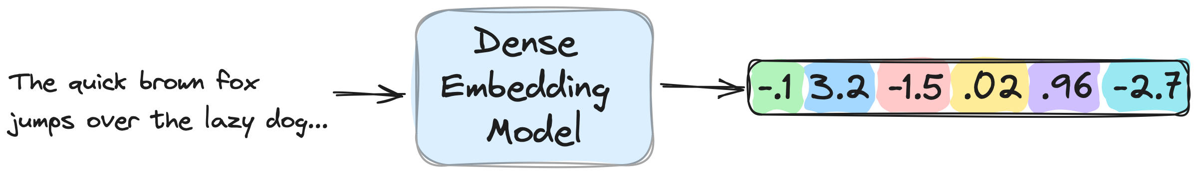
Notice the “dense” keyword in the figure? That’s because the output of the embedding model is a dense vector! In simple terms, a dense vector is a vector whose every entry is almost surely non-zero. While that is one of the most common types of embeddings you will encounter in the literature and in many applications, there is another type that offers unique and attractive properties: sparse embeddings. See Figure 2.

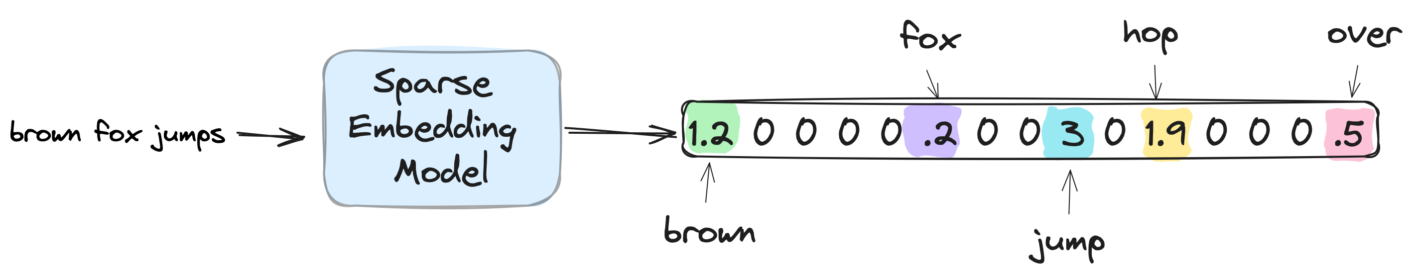
The focus of our paper (Bruch et al., 2024) is on these sparse representations. There are a number of reasons sparse embeddings are important enough to justify (our) research. Interpretability is one major factor: When every dimension corresponds to a term in some vocabulary, it is easy to understand what the embedding has extracted and captured from its input—“dictionary learning,” as it is sometimes known, is indeed a way to gain insight into large language models. In Figure 2, for example, the word “hop” has a non-zero weight, despite the fact that it does not appear in the input, though it is synonymous with “jump,” which does appear.

Inner Product as a measure of similarity

So we have defined how we represent text. Onto the second missing piece: How we define similarity. Considering our representation of text is in some vector space, it won’t surprise you to learn that similarity is measured by some notion of distance in vector spaces. Typical examples are the Euclidean distance, and, more commonly, angular distance or cosine similarity.

In our work, we consider a more general notion of similarity that includes the other two as special cases: inner product. If two vectors $u, v \in \mathbb{R}^d$ are $d$-dimensional vectors, then their inner product is $\langle u, v \rangle = \sum_{i=1}^d u_i v_i$ , where the subscript $i$ specifies the $i$-th coordinate.

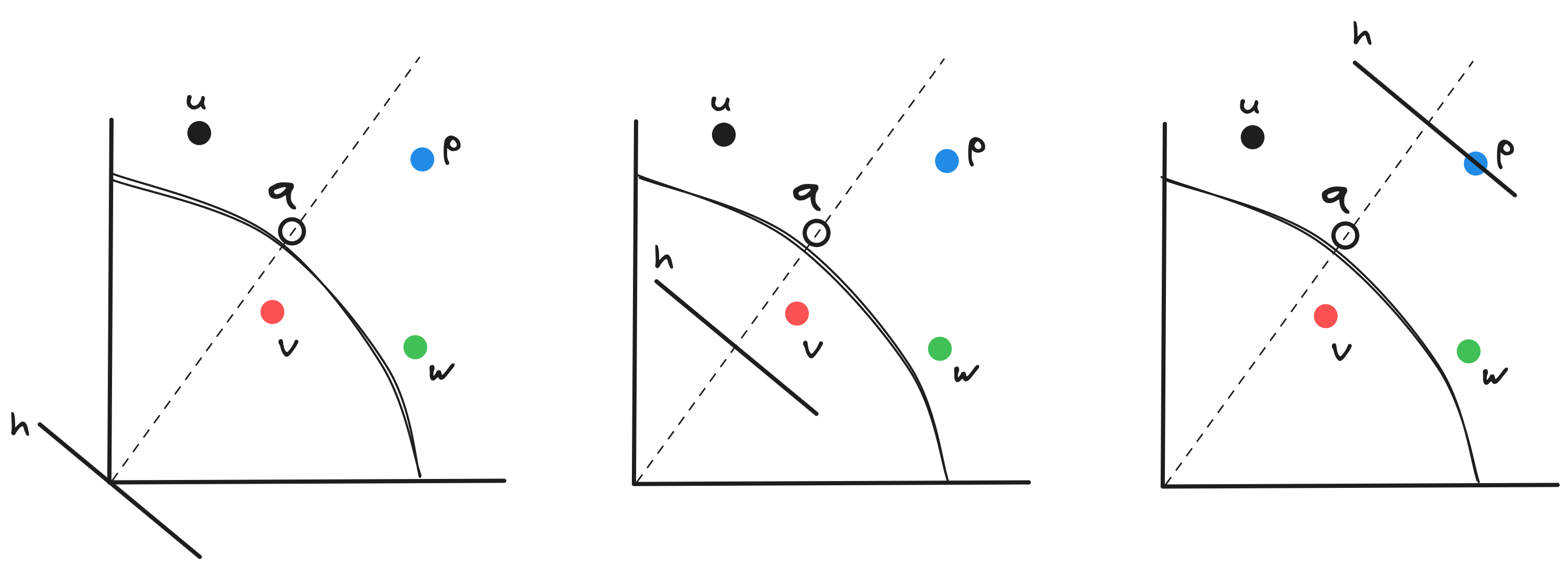
Let’s try to get a sense of what this means geometrically. In Figure 3, I plotted a few data points ($u, v, w$, and $p$) and a query point ($q$) in two dimensions. Which one of these data points has the largest inner product with $q$? The answer is $p$, but why? Take the direction of $q$ (i.e., the line from the origin that passes through $q$), and imagine the plane perpendicular to it ($h$). Start moving $h$ out towards infinity along the direction of $q$. The last point that touches $h$ maximizes inner product with $q$! This geometric interpretation extends naturally to higher dimensions too. Neat, no?!

Approximate Maximum Inner Product Search

While inner product is easy to define and wrap your head around, efficiently identifying a set of vectors that maximize the inner product with a query vector (i.e., $\argmax_u \langle q, u \rangle$ ) is, in general, hard in higher dimensions. There are many reasons why that is the case, which I will not get into here. If you are interested, you can find out why in my monograph on the subject (Bruch, 2024).

That is not to say we don’t have efficient ways of approximately solving the problem. That is, if we can tolerate a bit of error, then there are many classes of efficient algorithms that become relevant (Bruch, 2024). What “error” means is that, for a query $q$ , the set of $k$ points returned by an approximate algorithm may contain points whose inner product with $q$ may be smaller than the true $k$-th largest inner product. If $k=10$ , then maybe one point in the returned set is there erroneously, incorrectly replacing a true maximizer of inner product—in which case, the accuracy of our approximate algorithm would be $90\%$.

This relaxation helps us speed up retrieval. In fact, once you get in the right mindset that error is inevitable and that we can tolerate some degree of inaccuracy, then you can often trade off accuracy for speed, and vice versa! But how do we design an approximate algorithm? What properties of data can be leverage to approximately identify the solution to maximum inner product search, particularly in the context of learnt sparse embeddings? That finally brings us to what motivated our proposed method.

Concentration of mass

I often argue that a vector, any vector, is just a bunch of noise plus a bit of signal. I don’t claim this is original and don’t think it’s controversial either. That’s essentially the philosophy that powers much of the literature on sketching high-dimensional vectors (Woodruff, 2014) into low-dimensional subspaces—I’m being a bit handwavy, but hopefully you get the point.

We started from that philosophy and examined a number of benchmark retrieval datasets, including the MS MARCO Passage Retrieval collection embedded as sparse vectors with different flavors of the Splade model. What we observed is a manifestation of that philosophy: Most of the information represented by a sparse vector is concentrated in a few coordinates, with the rest amounting to noise. Let me elaborate.

Take a sparse embedding, say $u \in \mathbb{R}^d$ , from this family of models and look at its mass. Mass here means the $L_1$ norm: $\lVert u \rVert_1 = \sum_{i=1}^d \lvert u_i \rvert$. Now, sort the coordinates (the subscript $i$’s) by how much $u_i$’s contribute to the mass: The coordinate with the largest absolute value comes first, second largest second, and so on.

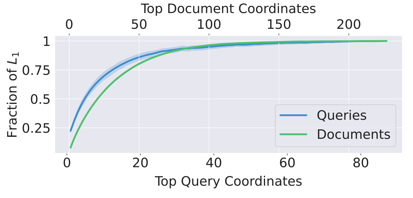
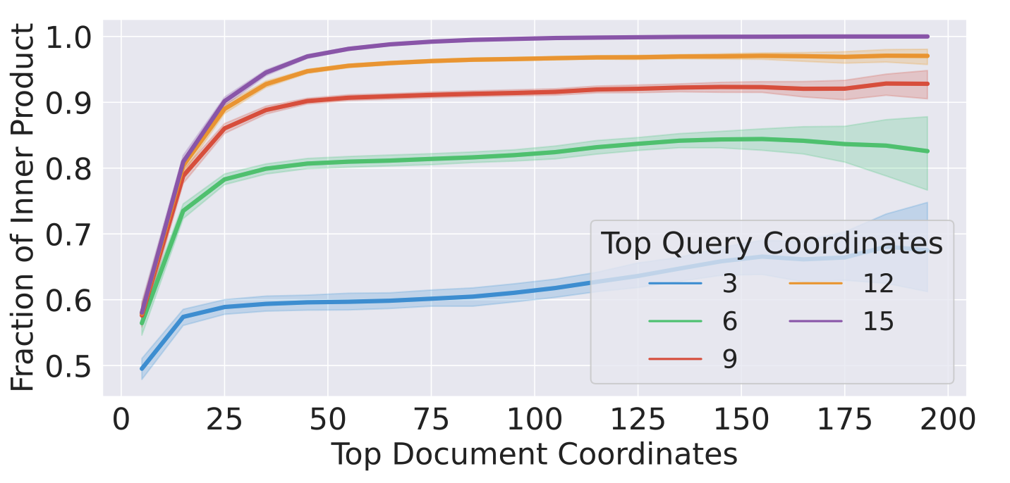
From this ordered list, collect the top $\kappa$ coordinates, and compute the partial sum of $\lvert u_i \rvert$’s corresponding to those coordinates. It should be obvious that as $\kappa$ gets larger, the partial sum converges to the $L_1$ norm of $u$. What is surprising, however, is that even when $\kappa$ is small (say, less than half of the total number of non-zero entries in $u$), we recover most of the $L_1$ mass anyway! This is what the left subfigure in Figure 4 illustrates.

That is what we expected to see. In fact, a similar observation based on the $L_2$ norm was recently developed into a very effective dimensionality reduction algorithm for sparse vectors (Daliri et al., 2024). Super!

Let me refer to a subvector made up of the top $\alpha$ fraction of coordinates of a vector, as its $\alpha$-mass subvector. It’s kind of a messy definition, but it makes talking about this business of ordering coordinates and taking the top fraction of them easier.

Back to our observation. What is perhaps even more interesting is that, if we take the inner product between the $\alpha$-mass subvector of a data point, with the $\beta$-mass subvector of a query, we can get arbitrarily close to the full inner product between the original vectors! That is what the right plot in Figure 4 shows: Partial inner product between the top 15 coordinates of a query with the top 75 coordinates of a document gives us almost all of the inner product between them.

This observation, which we called the “concentration of importance” (for consistency with IR jargon) gave us what we needed to design an approximate retrieval algorithm. Intuitively, we can throw away $(1-\alpha)$ fraction of data (and query) points and approximate the full inner product with arbitrary accuracy. So we have what we were looking for: a lever to control accuracy for speed. Next section explains how we take advantage of that property to design Seismic—our proposed algorithm.

Seismic

Seismic is a backronym that stands for Spilled Clustering of Inverted Lists with Summaries for Maximum Inner Product Search. Don’t ask me why, but our inside joke was that “the microsecond territory is shaking,” which led to this name for the algorithm—that name is one of my greatest accomplishments yet, and I’m famously not very creative with naming things!

If phrases like “spilled clustering” and “inverted lists” sound foreign, I will explain what they mean in a minute as I describe the two components of the algorithm: Indexing (data preprocessing) and retrieval (query processing or search). The rest of this section gives an intuitive construction of the data structures and the main algorithm that make up Seismic and were introduced more rigorously in our paper.

Index structure

Let me preface this section by noting that, generally speaking, more than 90% of the battle in designing a vector retrieval (or nearest neighbor search) algorithm is organizing the vectors into an index—although, in a recent paper (Bruch et al., 2024), we challenge that conventional wisdom. That is because, whether the index is a graph or a list of clusters with centroids, the retrieval algorithm is usually simple and greedy. So the right place to leverage the “concentration of importance” property is during indexing.

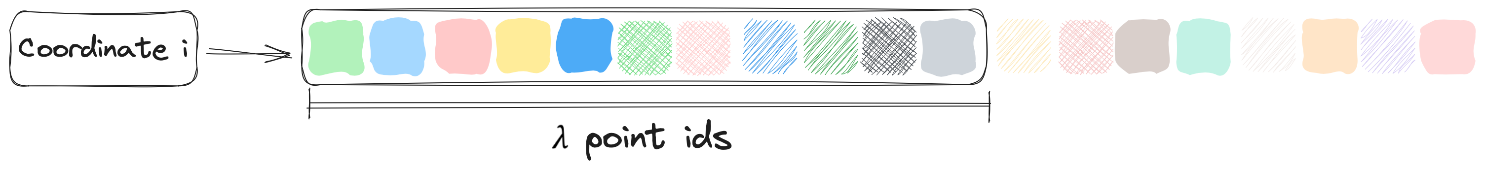
Seismic starts by building a good ol’ inverted index: A map that is keyed by coordinate index (the subscript $i$ in $u_i$), and where $i$ points to a list of vector ids whose $i$-th coordinate is non-zero. Each of those lists is called an inverted list, so that an inverted index is a mapping from coordinates to inverted lists. Historically, this data structure has been at the heart of sparse vector retrieval algorithms. This is what Figure 5 visualizes for a single coordinate.

In the first step of the algorithm, we truncate each inverted list and retain only the ids of $\lambda$ vectors with the largest $i$-th coordinate. That results in the structure in Figure 6.

How does this relate to the “concentration of importance” property? To understand that connection, it helps to visualize the vector collection as a matrix, as shown in Figure 7. In the figure, I’m plotting a matrix whose columns are data points and rows correspond to dimensions. White space represents zeros and the intensity of the shade of each block is supposed to convey the magnitude of each non-zero coordinate.

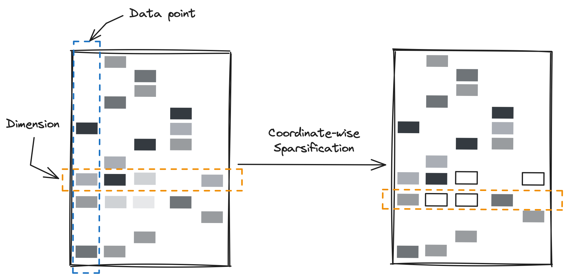
By truncating each inverted list (i.e., a row in the matrix), we discard entries from vectors conditioned on other vectors: $u_i$ can only be discarded if there are $\lambda$ other vectors with a larger $i$-th coordinate. In this way, one vector may turn into its $0.9$-mass subvector , another to $.2$-mass subvector , and another may remain completely intact. In other words, the importance of $u_i$ is determined not only relative to $\lVert u \rVert_1$ , but also relative to other vectors present in the collection.

Now that our inverted list for coordinate $i$ is truncated, we take the vectors corresponding to the $\lambda$ ids in the list, and apply geometric clustering (e.g., some variant of KMeans) to them. This results in $\beta$ groups of vector ids, whose vectors form partitions according to the clustering algorithm! This is visualized in Figure 8.

If this looks familiar to you, that’s probably because you know how clustering-based nearest neighbor search works! However, note that we apply clustering to each inverted list independently of other inverted lists. And because a vector id can appear in multiple inverted lists, it can therefore end up in multiple (overlapping) clusters. That is why we used the term “spilled clustering” (or spillage) to highlight this phenomenon.

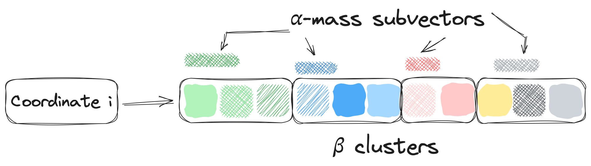
If you know about clustering-based indexes, you also know that each cluster is represented by a point, such as its centroid. Our index is no different. We equip each cluster (within an inverted list) with a representative point, called a “sketch” or “summary.” There are many ways to sketch a cluster such as the (coordinate-wise) mean of vectors, but in our work we choose to work with the following sketches: We first obtain the coordinate-wise maximum of all vectors present in a cluster, then take its $\alpha$-mass subvector as the final sketch! Schematically, this is what is presented in Figure 9.

Why maximum as opposed to mean? When $\alpha$ is large enough, coordinate-wise maximum gives a “bounding box” around the points within a cluster. In effect, inner product of an arbitrary query $q$ with any point in that cluster is necessarily smaller than the $\langle q, s \rangle$ if $s$ is the sketch. We will use this property during retrieval to dynamically skip clusters that have a low likelihood of containing the solution, where we assess that likelihood based on the inner product between the query and the cluster’s sketch.

That wraps up the index construction algorithm (i.e., Algorithm 1 in the paper). Note that, we introduce three tunable hyper-parameters:

• $\lambda$ : Truncation parameter. A smaller $\lambda$ leads to a sparser inverted index which presumably leads to accuracy degradation, whereas a larger value preserves more of the dataset, making search slower but more accurate.
• $\beta$ : Number of clusters in each inverted list. As $\beta \rightarrow \lambda$ , we form smaller clusters whose sketch would more accurately represent them, but because there are more clusters to process, search slows down.
• $\alpha$ : Determines the capacity of the $\alpha$-mass subvectors when forming cluster sketches. A larger $\alpha$ leads to a more complete sketch, with the property that the maximum inner product between a query and points in a cluster is less than the inner product between the query and the sketch. At the same time, larger values of $\alpha$ result in increased storage cost due to larger sketches.

These three parameters give us a way to control accuracy for speed. But to understand why exactly, we must turn to the retrieval algorithm itself. That’s the topic of the next section.

Retrieval procedure

Let’s say we have formed the index structure described in the preceding section, and are now ready to serve queries and return the top-$k$ set of vectors for every query. What now? The query processing procedure in Seismic is actually quite easy to explain. Let’s focus on a single query point for the sake of this discussion—queries are processed independently.

First, let’s initialize a heap that will contain pairs consisting of the id of a vector and its inner product with the query. The heap has a maximum capacity of $k$ elements, and has the invariant that, at any given time, the vectors present in the heap have the largest inner product with the query from among the vectors we have examined up to that time. At the end of the execution of the retrieval procedure, then, the top-$k$ set is contained in the heap.

The question now becomes: How do we populate the heap? To that end, we first order the non-zero coordinates of the query vector and keep cut number of the largest coordinates by absolute value—the result is a (cut$/|nnz(q)|$)-mass subvector where $|nnz(\cdot)|$ denotes the number of non-zero coordinates.

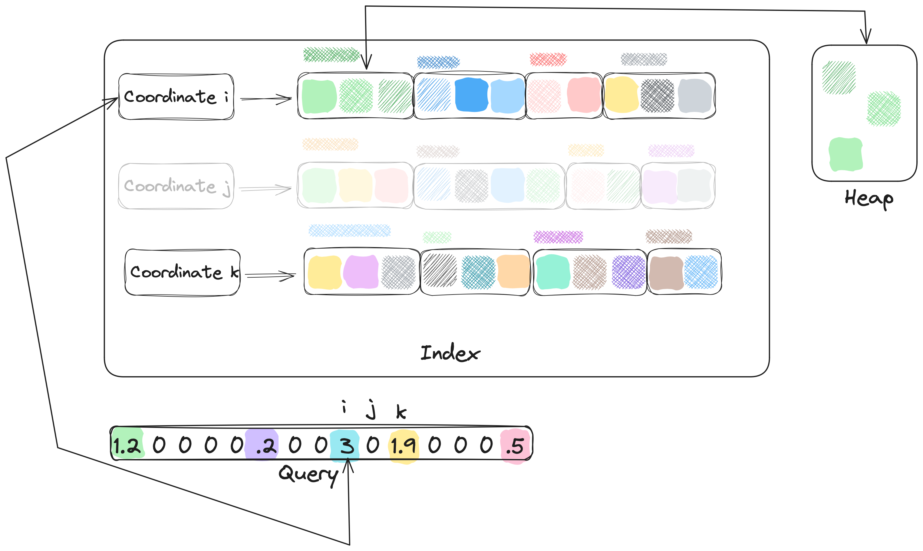
Take the largest coordinate (say, $i$) and look up its inverted list, as shown in Figure 10. Now, compute the inner product between the query and the sketch of the first cluster in the inverted list. If this inner product is smaller than the minimum inner product in the heap (scaled by a hyper-parameter called heap_factor), then we skip this cluster and move to the next. Otherwise, we grab the raw vectors whose ids are present in that cluster from storage, compute the true inner product between them and the full query vector, and insert each into the heap. Note that, when the heap grows past $k$ records, we simply drop the smallest values until there are at most $k$ vectors in it.

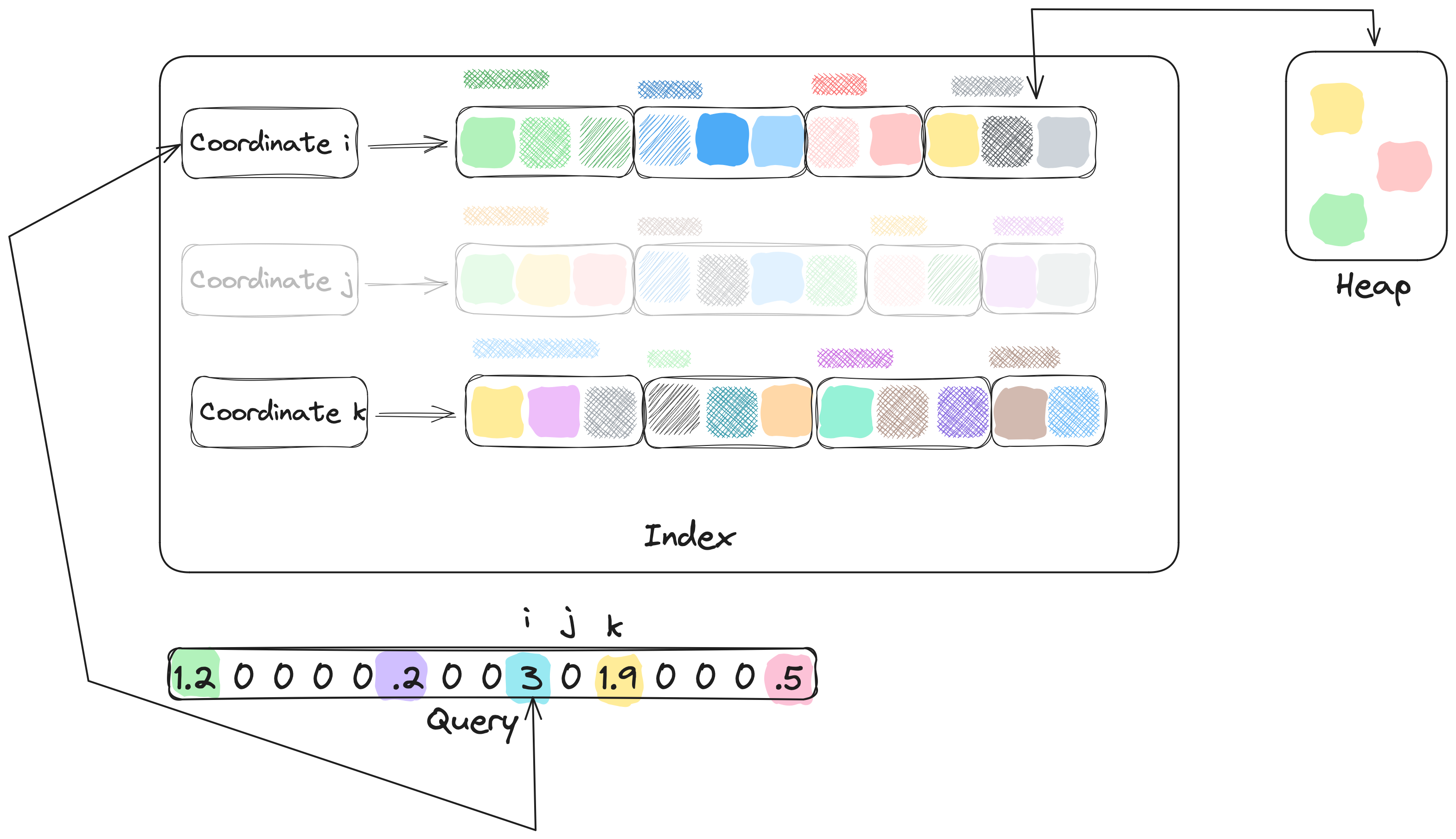
We repeat the procedure above for all clusters in the $i$-th list. When we processed the last cluster, the heap might look like what is depicted in Figure 11.

Finally, we repeat this entire procedure for every one of those cut query coordinates. That’s all there is to Seismic’s retrieval algorithm (i.e., Algorithm 2 in the paper)! Its relative efficiency, as shown by a variety of experiments in the paper, is the result of the fact that we dynamically skip over a large number of clusters when visiting each inverted list. That is so thanks to the sketches: We use the inner product between a query and a sketch to gauge how likely it is that a point in a cluster can out-score the vectors that are already present in the heap.

Summary of experiments

We put Seismic through a great deal of experiments and compared its performance against state-of-the-art sparse retrieval methods, from traditional inverted index-based solutions to graph-based approximate MIPS and more. We paid particular attention to accuracy, speed, index size, and index construction time, and studied their trade-offs.

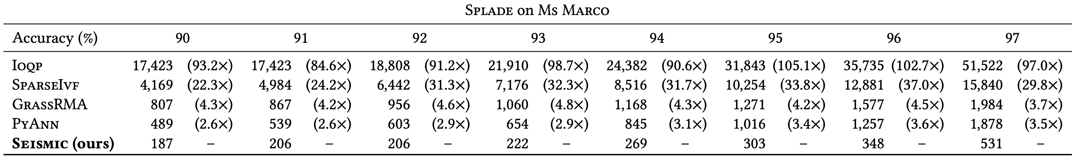
I refer you to the paper for a complete set of results and a detailed discussion, but I’d like to highlight one set of experiments in Figure 12, summarizing Seismic’s latency at various accuracy levels.

Resources

We have licensed our paper with Open Access (CC By 4.0), so you can read the camera-ready version directly off of ACM DL. We have also made our entire code base open source, which you can find in this repo. We are also committed to helping you reproduce our results, and are available to answer your questions; reach out, we are friendly, don’t be shy!

If you wish to cite our work, please use the following bibtex entry:

@inproceedings{bruch2024efficientinvertedindexesapproximate,
      author = {Bruch, Sebastian and Nardini, Franco Maria and Rulli, Cosimo and Venturini, Rossano},
      title = {Efficient Inverted Indexes for Approximate Retrieval over Learned Sparse Representations},
      year = {2024},
      url = {https://doi.org/10.1145/3626772.3657769},
      doi = {10.1145/3626772.3657769},
      booktitle = {Proceedings of the 47th International ACM SIGIR Conference on
                   Research and Development in Information Retrieval},
      pages = {152--162},
      numpages = {11},
      location = {Washington DC, USA},
}